1. reading a single VTU file

While beeing a python package, it is also tested in Julia, where it can be accessed via PyCall:

ENV["PYTHON"] = "/usr/bin/python3"
using Pkg
#Pkg.add("PyCall")
Pkg.build("PyCall")

using PyCall
@pyimport vtuIO

Single VTU files can be accessed via:

vtufile = vtuIO.VTUIO("examples/square_1e2_pcs_0_ts_1_t_1.000000.vtu", dim=2)

PyObject <vtuIO.VTUIO object at 0x7f3ccc65a760>

The dim argument is needed for correct interpolation. By defualt dim=3 is assumed. Basic VTU properties, like fieldnames, points and corresponding fielddata as provided by the unstructured grid VTK class can be simply accessed as follows:

fields=vtufile.get_point_field_names()

4-element Vector{String}:
 "D1_left_bottom_N1_right"
 "Linear_1_to_minus1"
 "pressure"
 "v"

vtufile.points[1:3]

3-element Vector{Float64}:
0
1
2

vtufile.get_point_field("v")

121×2 Matrix{Float64}:
0   0.0
0   1.62548e-16
0  -9.9123e-16
0  -9.39704e-16
0  -4.08897e-16
0   1.36785e-16
0  -3.23637e-16
0  -2.30016e-16
0  -7.69185e-16
0  -2.27994e-15
0   1.53837e-15
0   3.25096e-16
0  -3.62815e-16
 ⋮
0  -8.88178e-16
0   0.0
0  -2.22045e-16
0   9.9123e-16
0  -1.2648e-15
0   5.48137e-16
0  -3.89112e-17
0  -2.03185e-17
0  -1.02098e-15
0  -5.03586e-16
0  -3.37422e-15
0   8.88178e-16

Aside basic VTU properties, the field data at any given point, e.g., pt0 and pt1

points = Dict("pt0"=> (0.5,0.5,0.0), "pt1"=> (0.2,0.2,0.0))

Dict{String, Tuple{Float64, Float64, Float64}} with 2 entries:
  "pt1" => (0.2, 0.2, 0.0)
  "pt0" => (0.5, 0.5, 0.0)

can be retrieved via

point_data = vtufile.get_point_data("pressure", pts=points)

Dict{Any, Any} with 2 entries:
  "pt1" => 0.6
  "pt0" => 3.41351e-17

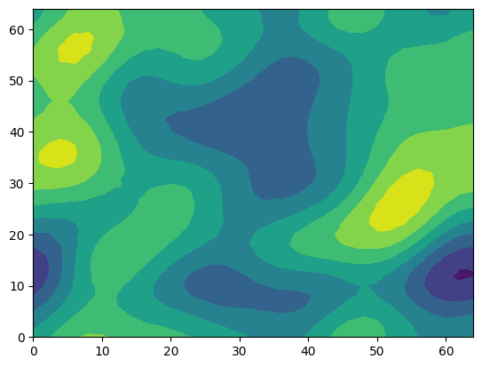
1.1 Creating contour plots

using PyPlot

vtufile = vtuIO.VTUIO("examples/square2d_random.vtu", dim=2)

PyObject <vtuIO.VTUIO object at 0x7f3ccc652220>

field = vtufile.get_point_field("gaussian_field_2");

triang = matplotlib.tri.Triangulation(vtufile.points[:,1], vtufile.points[:,2])

PyObject <matplotlib.tri.triangulation.Triangulation object at 0x7f3c7b057670>

tricontourf(triang,field)

PyObject <matplotlib.tri.tricontour.TriContourSet object at 0x7f3c76b14790>

This random field was created using the ranmedi package: https://github.com/joergbuchwald/ranmedi/

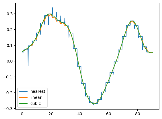
1.2 Extracting Pointsetdata

There are basically three interpolation methods available for extracting data at arbitrary points (cubic is only available for 1D and 2D). The default is linear.

methods = ["nearest", "linear", "cubic"];

diagonal = [(i,i,0) for i in 0:0.1:64];

vtufile = vtuIO.VTUIO("examples/square2d_random.vtu", dim=2)
data_diag = Dict()
for method in methods
    data_diag[method] = vtufile.get_point_set_data("gaussian_field_2", pointsetarray=diagonal, interpolation_method=method)
end

r_diag = sqrt.(first.(diagonal[:]).^2 + getindex.(diagonal[:],2).^2);

plot(r_diag, data_diag["nearest"], label="nearest")
plot(r_diag, data_diag["linear"], label="linear")
plot(r_diag, data_diag["cubic"], label="cubic")
legend()

PyObject <matplotlib.legend.Legend object at 0x7f3cccb83520>

2. Writing VTU files

some simple methods also exist for adding new fields to an existing VTU file or save it separately:

vtufile = vtuIO.VTUIO("examples/square_1e2_pcs_0_ts_1_t_1.000000.vtu", dim=2)

PyObject <vtuIO.VTUIO object at 0x7f3cccbb9190>

p_size = length(vtufile.get_point_field("pressure"))

p0 = ones(p_size) * 1e6;

vtufile.write_field(p0, "initialPressure", "mesh_initialpressure.vtu")

A new field can also created from a three-argument function for all space-dimensions:

function p_init(x,y,z)
    if x < 0.5
        return -0.5e6
    else
        return +0.5e6
    end
end

p_init (generic function with 1 method)

vtufile.func_to_field(p_init, "p_init", "mesh_initialpressure.vtu")

It is also possible to write multidimensional arrays using a function.

function null(x,y,z)
    return 0.0
end

null (generic function with 1 method)

vtufile.func_to_m_dim_field([p_init,p_init,null,null], "sigma00","mesh_initialpressure.vtu")

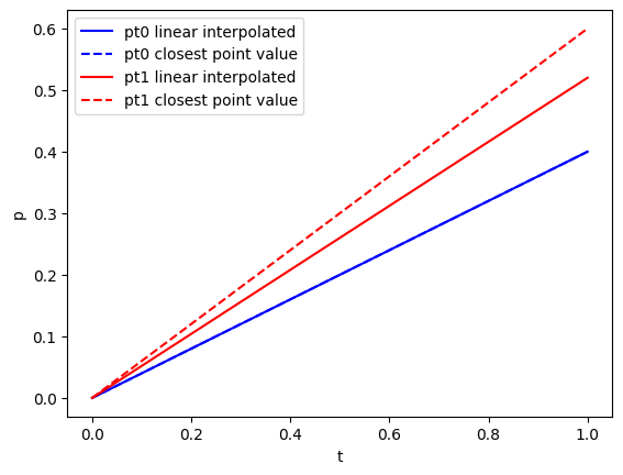
3. Reading time-series data from PVD files:

Similar to reading VTU files, it is possible extract time series data from a list of vtufiles given as a PVD file. For extracting grid data at arbitrary points within the mesh, there are two methods available. The stadard method is linear interpolation between cell nodes and the other is the value of the closest node:

pvdfile = vtuIO.PVDIO("examples/square_1e2_pcs_0.pvd", dim=2)

PyObject <vtuIO.PVDIO object at 0x7f3cccbf1550>

Timesteps can be obtained through the timesteps instance variable:

time = pvdfile.timesteps

2-element Vector{Float64}:
 0.0
 1.0

points = Dict("pt0"=> (0.3,0.5,0.0), "pt1"=> (0.24,0.21,0.0))

Dict{String, Tuple{Float64, Float64, Float64}} with 2 entries:
  "pt1" => (0.24, 0.21, 0.0)
  "pt0" => (0.3, 0.5, 0.0)

pressure_linear = pvdfile.read_time_series("pressure", points)

Dict{Any, Any} with 2 entries:
  "pt1" => [0.0, 0.52]
  "pt0" => [0.0, 0.4]

pressure_nearest = pvdfile.read_time_series("pressure", points, interpolation_method="nearest")

Dict{Any, Any} with 2 entries:
  "pt1" => [0.0, 0.6]
  "pt0" => [0.0, 0.4]

using Plots

As point pt0 is a node in the mesh, both values at $t=1$ agree, whereas pt1 is not a mesh node point resulting in different values.

plot(time, pressure_linear["pt0"], "b-", label="pt0 linear interpolated")
plot(time, pressure_nearest["pt0"], "b--", label="pt0 closest point value")
plot(time, pressure_linear["pt1"], "r-", label="pt1 linear interpolated")
plot(time, pressure_nearest["pt1"], "r--", label="pt1 closest point value")
legend()
xlabel("t")
ylabel("p")

PyObject Text(24.000000000000007, 0.5, 'p')

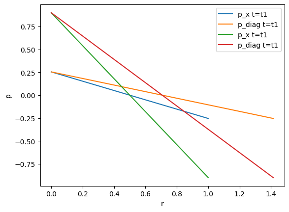
4. Reading point set data from PVD files

Define two discretized axes:

xaxis =  [(i,0,0) for i in 0:0.01:1]
diagonal = [(i,i,0) for i in 0:0.01:1];

The data along these axes should be extracted at two arbitrary distinct times (between the existing timeframes t=0.0 and t=1):

t1 = 0.2543
t2 = 0.9

0.9

pressure_xaxis_t1 = pvdfile.read_set_data(t1, "pressure", pointsetarray=xaxis);
pressure_diagonal_t1 = pvdfile.read_set_data(t1, "pressure", pointsetarray=diagonal);
pressure_xaxis_t2 = pvdfile.read_set_data(t2, "pressure", pointsetarray=xaxis);
pressure_diagonal_t2 = pvdfile.read_set_data(t2, "pressure", pointsetarray=diagonal);

r_x = first.(xaxis[:]);

r_diag = sqrt.(first.(diagonal[:]).^2 + getindex.(diagonal[:],2).^2);

plot(r_x, pressure_xaxis_t1, label="p_x t=t1")
plot(r_diag, pressure_diagonal_t1, label="p_diag t=t1")
plot(r_x, pressure_xaxis_t2, label="p_x t=t1")
plot(r_diag, pressure_diagonal_t2, label="p_diag t=t1")
xlabel("r")
ylabel("p")
legend()

PyObject <matplotlib.legend.Legend object at 0x7f3c5f4d19d0>